Table of content:

What is XYZ?

Understand some foundational terms in machine learning area will help you to speed up the communication with experts. There are some famous terms you have to know.

Basic terms

What is loss, cost, objective function?

These are not very strict terms and they are highly related. However: In short, a loss function is a part of a cost function which is a type of an objective function.

From section 4.3 in “Deep Learning” - Ian Goodfellow, Yoshua Bengio, Aaron Courville http://www.deeplearningbook.org/ The function we want to minimize or maximize is called the objective function, or criterion. When we are minimizing it, we may also call it the cost function, loss function, or error function.

Loss function

A loss function is a way to map the performance of our model into a real number. It measures how well the model is performing its task.

It is usually a function defined on a data point, prediction and label, and measures the penalty. For example: square loss $l(f(x_i\vert θ),y_i)=(f(x_i\vert θ)−y_i)^2$ , used in linear regression hinge loss $l(f(x_i\vert θ),y_i)=max(0,1−f(x_i\vert θ)y_i)$ , used in SVM 0/1 loss $l(f(x_i\vert θ),y_i)=1⟺f(x_i\vert θ)≠y_i$ , used in theoretical analysis and definition of accuracy

Cost function

It is usually more general. It might be a sum of loss functions over your training set plus some model complexity penalty (regularization). For example: Mean Squared Error $MSE(θ)=\frac{1}{N} \sum_{i=1}^n(f(x_i\vert θ)−y_i)^2$ SVM cost function $SVM(θ)=∥θ∥^2+C\sum_{i=1}^nξ_i$ (there are additional constraints connecting ξi with C and with training set)

Objective function

It is the most general term for any function that you optimize during training. For example, a probability of generating training set in maximum likelihood approach is a well defined objective function, but it is not a loss function nor cost function (however you could define an equivalent cost function). For example: MLE is a type of objective function (which you maximize) Divergence between classes can be an objective function but it is barely a cost function, unless you define something artificial, like 1-Divergence, and name it a cost

What is the loss function of linear regression?

Mean Squared Error, or L2 loss. Given our simple linear equation y=mx+b, we can calculate MSE as:

$MSE = \frac{1}{N}\sum_{i=1}^n(y_i - (mx_i + b))^2$

N is the total number of data

$y_i$ is the actual data

$mx_i + b$ is our prediction

def MSE(yHat, y):
    return np.sum((yHat - y)**2) / y.size

What is the loss function of logistic regression?

Cross-Entropy

In binary classification, where the number of classes M equals 2, cross-entropy can be calculated as:

$Binary Cross Entropy = −(ylog(p)+(1−y)log(1−p))$ $Cross Entropy = -\sum_{c=1}^M y_{o,c}log(p_{o,c})$

M - number of classes (dog, cat, fish)

log - the natural log

y - binary indicator (0 or 1) if class label

c is the correct classification for observation o

p - predicted probability observation o is of class c

def CrossEntropy(yHat, y):
    if y == 1:
      return -log(yHat)
    else:
      return -log(1 - yHat)

Optimization of model

What is L1 regularizer?

Reference: Differences between L1 and L2 as Loss Function and Regularization

A regression model that uses L1 regularization technique is called Lasso Regression.

Lasso Regression (Least Absolute Shrinkage and Selection Operator) adds “absolute value of magnitude” of coefficient as penalty term to the loss function. Lasso shrinks the less important feature’s coefficient to zero thus, removing some feature altogether. So, this works well for feature selection in case we have a huge number of features.

$w^* = \underset{w}argmin\sum_j^n (t(x_i)-\sum_i^k w_i h_i(x_j))^2 + \lambda \sum_{i=1}^k \vert w_i\vert$

What is L2 regularizer?

Reference: Differences between L1 and L2 as Loss Function and Regularization

A regression model which uses L2 is called Ridge Regression.

Ridge regression adds “squared magnitude” of coefficient as penalty term to the loss function.

$w^* = \underset{w}argmin\sum_j^n (t(x_i)-\sum_i^k w_i h_i(x_j))^2 + \lambda \sum_{i=1}^k (w_i)^2$

What is imbalance data?

Reference: imbalanced data

Imbalanced data typically refers to a classification problem where the number of observations per class is not equally distributed; often you’ll have a large amount of data/observations for one class (referred to as the majority class), and much fewer observations for one or more other classes (referred to as the minority classes)

Two common ways we’ll train a model: tree-based logical rules developed according to some splitting criterion, and parameterized models updated by gradient descent.

It’s worth noting that not all datasets are affected equally by class imbalance. Generally, for easy classification problems in which there’s a clear separation in the data, class imbalance doesn’t impede on the model’s ability to learn effectively. However, datasets that are inherently more difficult to learn from see an amplification in the learning challenge when a class imbalance is introduced.

What are metrics to evaluate a model for imbalance data

Accuracy is not a good metrics for imbalance data. The model always predict the negative (majority) cases will get high accuracy.

Below are better metrics:

TP (True Positive), FP (False Positive), TN (True Negative), FN
Precision and recall
F1 or $F_{\beta}$

We can roughly classify the approaches into three major categories: cost function based approaches, sampling based approaches and turning the task to Anomaly detections.

Cost function based approaches

Reference: class-imbalance-problem

One of the simplest ways to address the class imbalance is to simply “provide a weight for each class” which places more emphasis on the minority classes such that the end result is a classifier which can learn equally from all classes.

The intuition behind cost function based approaches is that if we think one false negative is worse than one false positive, we will count that one false negative as, e.g., 100 false negatives instead. For example, if 1 false negative is as costly as 100 false positives, then the machine learning algorithm will try to make fewer false negatives compared to false positives (since it is cheaper).

Sampling based approaches

Another approach towards dealing with a class imbalance is to simply alter the dataset to remove such an imbalance.

This can be roughly classified into three categories:

Oversampling, by adding more of the minority class so it has more effect on the machine learning algorithm
Undersampling, by removing some of the majority class so it has less effect on the machine learning algorithm
Hybrid, a mix of oversampling and undersampling

Oversampling

Oversampling the minority classes to increase the number of minority observations until we’ve reached a balanced dataset.

Random oversampling

The most naive method of oversampling is to randomly sample the minority classes and simply duplicate the sampled observations. With this technique, it’s important to note that you’re artificially “reducing the variance” of the dataset.

Synthetic Minority Over-sampling Technique (SMOTE)

SMOTE is a technique that generates new observations by interpolating between observations in the original dataset.

For a given observation $x_i$ , a new (synthetic) observation is generated by interpolating between one of the k-nearest neighbors, $x_{zi}$ .

$x_{new} = x_i + \lambda (x_{zi}−x_i)$ where λ is a random number in the range [0,1]. This interpolation will create a sample on the line between $x_i$ and $x_{zi}$ .

This algorithm has three options for selecting which observations, $x_i$ , to use in generating new data points.

regular: No selection rules, randomly sample all possible $x_i$ .
borderline: Separates all possible $x_i$ into three classes using the k nearest neighbors of each point.

a. noise: all nearest-neighbors are from a different class than $x_i$

b. in danger: at least half of the nearest neighbors are of the same class as $x_i$

c. safe: all nearest neighbors are from the same class as $x_i$
svm: Uses an SVM classifier to identify the support vectors (samples close to the decision boundary) and samples $x_i$ from these points.

Adaptive Synthetic (ADASYN)

Adaptive Synthetic (ADASYN) sampling works in a similar manner as SMOTE, however, the number of samples generated for a given $x_i$ is proportional to the number of nearby samples which “do not” belong to the same class as $x_i$ . Thus, ADASYN tends to focus solely on outliers when generating new synthetic training examples.

Undersampling

To achieve class balance by undersampling the majority class - essentially throwing away data to make it easier to learn characteristics about the minority classes.

Random undersampling

A naive implementation would be to simply sample the majority class at random until reaching a similar number of observations as the minority classes.

For example, if your majority class has 1,000 observations and you have a minority class with 20 observations, you would collect your training data for the majority class by randomly sampling 20 observations from the original 1,000. As you might expect, this could potentially result in removing key characteristics of the majority class.

Near miss

reference: Illustration of the sample selection for the different NearMiss algorithms

The general idea behind near miss is to only the sample the points from the majority class necessary to distinguish between other classes.

NearMiss-1

Select samples from the majority class for which the average distance of the N closest samples of a minority class is smallest.

NearMiss1

NearMiss-2

Select samples from the majority class for which the average distance of the N farthest samples of a minority class is smallest.

NearMiss2

NearMiss-3

NearMiss-3 is a 2-steps algorithm. First, for each negative sample, their M nearest-neighbors will be kept. Then, the positive samples selected are the one for which the average distance to the N nearest-neighbors is the largest. NearMiss3

Tomeks links

Tomek’s link exists if two observations of different classes are the nearest neighbors of each other.

We’ll remove any observations from the majority class for which a Tomek’s link is identified

Depending on the dataset, this technique won’t actually achieve a balance among the classes - it will simply “clean” the dataset by removing some noisy observations, which may result in an easier classification problem.

Most classifiers will still perform adequately for imbalanced datasets as long as there’s a clear separation between the classifiers. Thus, by focusing on removing noisy examples of the majority class, we can improve the performance of our classifier even if we don’t necessarily balance the classes.

Edited nearest neighbors

Edited Nearest Neighbors applies a nearest-neighbors algorithm and “edit” the dataset by removing samples which do not agree “enough” with their neighborhood.

For each sample in the class to be under-sampled, the nearest-neighbors are computed and if the selection criterion is not fulfilled, the sample is removed.

This is a similar approach as Tomek’s links in the respect that we’re not necessarily focused on actually achieving a class balance, we’re simply looking to remove noisy observations in an attempt to make for an easier classification problem.

Hybrid approach

By combining undersampling and oversampling approaches, we get the advantages but also drawbacks of both approaches as illustrated above, which is still a tradeoff.

What is Anomaly Detection?

Reference:

Anomaly Detection

Anomaly Detection Algorithm

Dealing with Imbalanced Classes in Machine Learning

When you positive data is extremely small (2~20 or less than 50), throw away minority examples and switch to an anomaly detection framework. Assume you have 10000 data, only 20 positive data. You can select 6000 negative data to form a training set. Leverage gaussian distribution on each feature to form a probability model. Then set up an error probability = e, then P( $x_test$ ) < e will be an anomaly case. Assume each feature $x_i$ are independent and its values fellow gaussian distribution.

P(X) = P( $x_1$ ; $\mu_1$ ; $\sigma_1^2$ ) * P( $x_2$ ; $\mu_2$ ; $\sigma_2^2$ ) * … * P( $x_n$ ; $\mu_n$ ; $\sigma_n^2$ )

We can plot histogram for each feature to verify its distribution. If it does not follow gaussian distribution, we need to transform the feature to new feature.

example:

$x_{new1}$ = log( $x_1$ )

$x_{new2}$ = $x_2^{0.05}$

What is Receiver Operating Characteristics (ROC) curve?

Reference: imbalanced data

An ROC curve visualizes an algorithm’s ability to discriminate the positive class from the rest of the data. We’ll do this by plotting the True Positive Rate against the False Positive Rate for varying prediction thresholds.

$TPR = \frac{True Positives}{True Positives + False Negatives}$ $FPR = \frac{False Positives}{False Positives + True Negatives}$

What is the area under the curve (AUC)?

Reference: imbalanced data

The area under the curve (AUC) is a single-value metric for which attempts to summarize an ROC curve to evaluate the quality of a classifier. This metric approximates the area under the ROC curve for a given classifier. The ideal curve hugs the upper left hand corner as closely as possible, giving us the ability to identify all true positives while avoiding false positives; this ideal model would have an AUC of 1. On the flipside, if your model was no better than a random guess, your TPR and FPR would increase in parallel to one another, corresponding with an AUC of 0.5.

What is p value?

The P value, or calculated probability, is the probability of finding the observed, or more extreme, results when the null hypothesis ( $H_0$ ) of a study question is true – the definition of ‘extreme’ depends on how the hypothesis is being tested. P is also described in terms of rejecting $H_0$ when it is actually true, however, it is not a direct probability of this state.

What is TF-IDF?

Term Frequency–Inverse Document Frequency

Term Frequency also known as TF measures the number of times a term (word) occurs in a document.

$tf(t,d) = \frac{f_{t,d}}{\sum_{t'\in{d}}f_{t',d}}$

The inverse document frequency is a measure of how much information the word provides, that is, whether the term is common or rare across all documents.

$idf(t, D) = log \frac{N}{\vert {d\in{D}: t\in{d}} \vert}$

N: total number of documents in the corpus N = |D|
$\vert {d\in{D}: t\in{d}}\vert$ : number of documents where the term t appears. if the term is not in the corpus, this will lead to a division-by-zero. It is therefore common to adjust the denominator to 1+ $\|{d\in{D}: t\in{d}}\|$

$tfidf(t,d, D) = tf(t, d) * idf(t, D)$

What is Bias?

The bias of an estimator $\hat{\theta_m}$ to a statistic model $\theta$ is:

$Bias(\hat{\theta_m}) = E(\hat{\theta_m}) - \theta$

$\theta$ is the true underlying value of $\theta$ used to define the data generating distribution.

$E(\hat{\theta_m})$ is the expectation over the data (seen as samples from a random variable) by an estimator $\hat{\theta_m}$ .

In a simulation experiment concerning the properties of an estimator, the bias of the estimator may be assessed using the mean signed difference (ignore the noise for estimation purpose).

Mean Signed Difference, Deviation or Error (MSD)

$B = Mean Signed Diviation/Difference + Irreducible Error = MSD(\hat{\theta}) + noise = \frac{1}{n}\sum_{j=1}^n(\hat{\theta_j} - \theta_i) + noise$

The bias is an error from erroneous assumptions in the learning algorithm. High bias can cause an algorithm to miss the relevant relations between features and target outputs (underfitting).

Bias occurs when an algorithm has limited flexibility or is not complex enough produce underfit model that can’t learn the true signal from a dataset.

High bias, low variance algorithms train models that are consistent, but inaccurate on average. Small gap between training and test error but unacceptable high training error in high bias cases.

Try a larger set of features, less regularization, unpruned trees, small-k KNN to fix high bias/small variance issue.

What is Variance?

The variance is an error from sensitivity to small fluctuations in the training set. High variance can cause an algorithm to model the random noise in the training data, rather than the intended outputs (overfitting).

The variance of an estimator is simply the variance

$Var(\hat{\theta}) = \frac{\sum(x_i-\bar{x})^2}{n}$ (Machine Learning usually uses biased Variance)

$Var(\hat{\theta}) = \frac{\sum(x_i-\bar{x})^2}{n-1}$ (Statistic usually uses unbiased Variance)

Alternately, the square root of the variance is called the standard error, denoted $SE(\hat{\theta})$ .

Variance refers to an algorithm’s sensitivity to specific sets of training data. Algorithms are too complex produce overfit models that memorize the noise instead of the signal.

High variance, low bias algorithms train models that are accurate on average, but inconsistent. Test error still decreasing as training set size increase but large gap between training and test error. Suggests larger training set will help.

Try to get more training examples, highly regularized, highly pruned decision, large K KNN or try a smaller set of features to fix high variance/small bias issue.

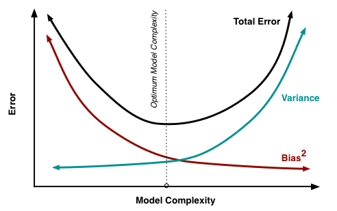
What is Bias-Variance tradeoff?

To get good predictions, you’ll need to find a balance of bias and variance that minimizes “total error”.

What is Bias-Variance decomposition of error?

Assume that $Y = f(X) + \epsilon = 0$ where $E(\epsilon) = 0$ and $Var(\epsilon) = \sigma_{\epsilon}^2$ , we can derive an expression for the expected prediction error of a regression fit $\hat{f}(X)$ at an input point $X = x_0$ , using squared-error loss:

$Err(x_0) = E[(Y-\hat{f}(x_0))^2 \vert X = x_0]\\ = [E\hat{f}(x_0)-f(x_0)] + E[\hat{f}(x_0)-E\hat{f}(x_0)]^2 + \sigma_{\epsilon}^2\\ = Bias^2(\hat{f}(x_0)) + Var(\hat{f}(x_0)) + Irreducible Error\\ = Bias^2 + Variance + Irreducible Error$

Irreducible error is “noise” that can’t be reduced by algorithm. It can sometimes be reduced by better data cleaning.

Low variance algorithms tend to be less complex, with simple or rigid underlying structure.

Examples:

Regression, Naive Bayes, Linear algorithms, parametric algorithms.

Low bias algorithms tend to be more complex, with flexible underlying structure.

Examples:

Decision trees, nearest neighbors, non-linear algorithms, non-parametric algorithms.

A proper machine learning workflow finds that optimal balance.

Separate training and test sets.
Trying appropriate algorithms
Fitting model parameters
Tunning impactful hyperparameters
Proper performance metrics
Systematic cross-validation

Bias-VarianceTradeOff

training and validation error

High bias and low bias case

high variance and low variance case

Diagnostic:

–Variance: Training error will be much lower than test error.

–Bias: Training error will also be high.

Reference:

What is Recurrent Neural Networkn (RNN)?

A recurrent neural network (RNN) is a class of artificial neural network where connections between nodes form a directed graph along a sequence. This allows it to exhibit dynamic temporal behavior for a time sequence. This allows it to exhibit dynamic temporal behavior for a time sequence. RNNs can use their internal state (memory) to process sequences of inputs.

In other neural networks, all the inputs are independent of each other. But in RNN, all the inputs are related to each other. RNNs are called recurrent because they perform the prediction task for every element of a sequence, with the output being depended on the previous computations.

What are main gates in Long Short-Term Memory (LSTM)?

Long short-term memory (LSTM) units are units of a recurrent neural network (RNN). An RNN composed of LSTM units is often called an LSTM network. A common LSTM unit is composed of a cell, an input gate, an output gate and a forget gate. The cell remembers values over arbitrary time intervals and the three gates regulate the flow of information into and out of the cell.

What is (Support Vector Machine) SVM?

SVM is supervised learning models with associated learning algorithms that analyze data used for classification and regression analysis.

Hard-margin

If the training data is linearly separable, we can select two parallel hyperplanes that separate the two classes of data, so that the distance between them is as large as possible. The region bounded by these two hyperplanes is called the “margin”, and the maximum-margin hyperplane is the hyperplane that lies halfway between them.

An important consequence of this geometric description is that the max-margin hyperplane is completely determined by those $\overrightarrow{x_i}$ which lie nearest to it. These $\overrightarrow{x_i}$ are called support vectors.

Soft-margin

To extend SVM to cases in which the data are not linearly separable, we introduce the hinge loss function:

$max(0, 1-y_i(\overrightarrow{w}*\overrightarrow{x_i}-b))$ is the current output.

If $\overrightarrow{x_i}$ lies on the correct side of the margin, the loss function is zero.

Note that $y_i$ is the ith target(i.e., in this case, 1 or -1), and $(\overrightarrow{w}*\overrightarrow{x_i}-b)$

We then wish to minimize

$[\frac{1}{n}\sum_{i=1}^n max(0, 1-y_i(\overrightarrow{w}*\overrightarrow{x_i}-b))] + \lambda \|\overrightarrow{w}^2\|$

where the parameter $\lambda$ determines the tradeoff between increasing the margin-size and ensuring that the $\overrightarrow{x_i}$ lie on the correct side of the margin.

What is Entropy in discrete?

$H(p) = -\sum_x p(x) log p(x)$

What is Cross Entropy in discrete?

$H(p, q) = -\sum_x p(x) log q(x)$ or by definition: $H(p, q) = H(p) + D_{KL}(p \vert\vert q)$

What is the difference between Cross Entropy and Entropy?

The KL divergence from $\hat{y}$ (or Q, your observation) to y (or P, ground truth) is simply the difference between cross entropy and entropy:

$KL(y \vert\vert \hat{y})=\sum_iy_ilog\frac{1}{\hat{y}_i}−\sum_iy_ilog\frac{1}{y_i}=\sum_iy_ilog\frac{y_i}{\hat{y}_i}$

What is Post-of-Speech (POS) Tagging in NLP?

How to do the POS tagging?

Use of hidden Markov models

Dynamic programming methods

Unsupervised taggers

Other taggers and methods

include the Viterbi algorithm, Brill tagger, Constraint Grammar, and the Baum-Welch algorithm (also known as the forward-backward algorithm)

Hidden Markov model and visible Markov model taggers can both be implemented using the Viterbi algorithm.

What is the loss function in mathematics?

What is Conditional Random Field?

Reference: Overview of Conditional Random Fields

Introduction to Conditional Random Fields

What is XYZ?

Basic terms

What is loss, cost, objective function?

Loss function

Cost function

Objective function

What is the loss function of linear regression?

What is the loss function of logistic regression?

Optimization of model

What is L1 regularizer?

What is L2 regularizer?

What is imbalance data?

What are metrics to evaluate a model for imbalance data

Cost function based approaches

Sampling based approaches

Oversampling

Random oversampling

Synthetic Minority Over-sampling Technique (SMOTE)

Adaptive Synthetic (ADASYN)

Undersampling

Random undersampling

Near miss

NearMiss-1

NearMiss-2

NearMiss-3

Tomeks links

Edited nearest neighbors

Hybrid approach

What is Anomaly Detection?

What is Receiver Operating Characteristics (ROC) curve?

What is the area under the curve (AUC)?

What is p value?

What is TF-IDF?

What is Bias?

Mean Signed Difference, Deviation or Error (MSD)

What is Variance?

What is Bias-Variance tradeoff?

What is Bias-Variance decomposition of error?

What is Recurrent Neural Networkn (RNN)?

What are main gates in Long Short-Term Memory (LSTM)?

What is (Support Vector Machine) SVM?

Hard-margin

Soft-margin

What is Entropy in discrete?

What is Cross Entropy in discrete?

What is the difference between Cross Entropy and Entropy?

What is Post-of-Speech (POS) Tagging in NLP?

How to do the POS tagging?

Use of hidden Markov models

Dynamic programming methods

Unsupervised taggers

Other taggers and methods

What is the loss function in mathematics?

What is Conditional Random Field?

What is the meaning of Conditional in this algorithm?

How CRFs differ from Hidden Markov Models

What is the relationship between Hidden Markov Model and Conditional Random Field?

What is Viterbi algorithm

What is Jaccard Similarity

What is MinHash

What is Locality Sensitive Hashing(LSH)

What is Shingling